The Sound of Emergence

Life in a (non) analytical world

Imagine taking a glass of water at room temperature and cooling it by 1 degree. At first glance, the system would look almost identical, beyond feeling slightly colder when touched. At a second glance, a physicist or a chemist might be able to measure some differences in a set of measurable quantities such as the heat capacity, but overall the intensity of these changes would be proportional to the decrease in temperature.

Indeed in ordinary life we expect physical laws to be well behaved: we have internalised the idea that the effects of an action are generically proportionate to its intensity, that observables do not change abruptly but vary continuously. Let us call the world that evolves under these expectations analytic.

Now repeat the same experiment with a glass of water that sits right above the freezing temperature. Your faith in analyticity will be torn apart. Everything about the object changes at once: its rigidity, its density, the way it reflects and absorbs light. A small change in temperature has produced a huge physical transformation.

These types of phenomena, called Phase Transitions, have fascinated physicists for centuries, precisely because of their non-analyticities. They cannot be understood from the individual properties of the atoms alone, but require an understanding of the interaction between many such atoms, and are therefore an example of emergent phenomena.

In this article, we will explore some of the most striking properties of phase transitions, using the Ising Model as our prototypical example. We will examine how its properties change not only from a visual perspective but also an auditory one, using the art of data sonification to translate key parameters of the model into sound.

The Ising Model

At the end of the XIX century, the French physicist Pierre Curie described a new phase transition: he observed that certain materials, below a certain temperature (which varies across materials), acquired spontaneous magnetisation. In an attempt to explain the core mechanism of this transition, in 1925 a German physicist called Ernst Ising proposed a model which now bears his name.

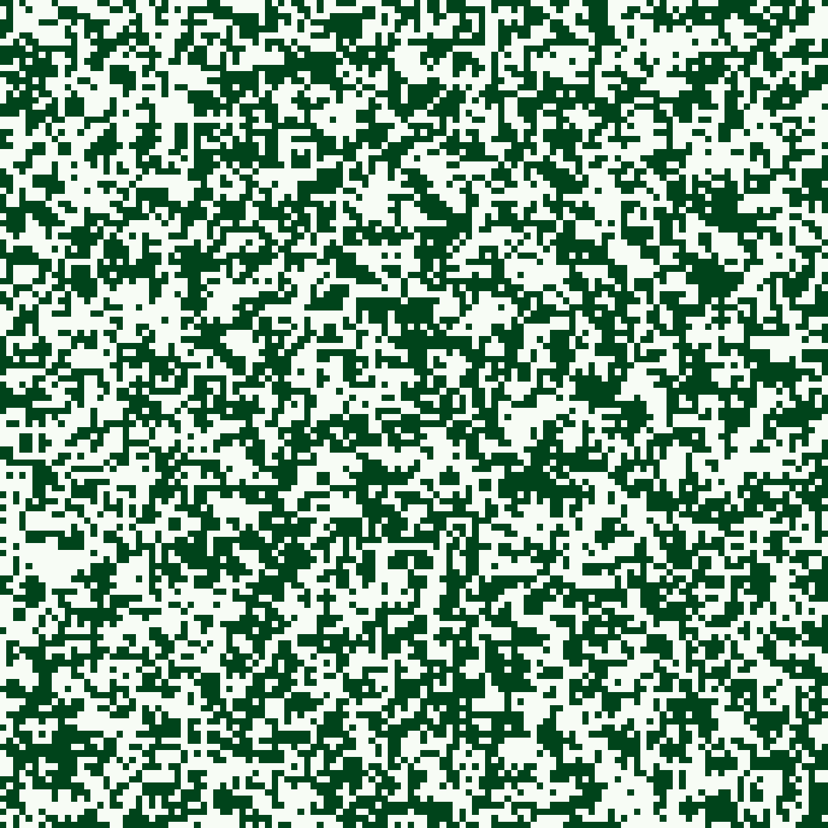
The Ising Model is an extremely simplified model of magnetism: it is defined on a 2d grid of pixels, where each pixel can be in one of two states, “up” or “down”, representing the orientation of a tiny magnetic spin. Each spin interacts only with its immediate neighbours, and the interaction prefers alignment: neighbouring spins lower their energy by pointing the same way. The parameter that controls the strength of this alignment preference is the temperature T, low temperature corresponding to a high alignment strength and vice versa.

The macroscopic state of the model is captured by an observable called the magnetisation m. It is defined as the number of “up” spins minus the number of “down” spins, divided by the total amount of spins. When there are roughly the same amount of up and down spins m = 0, and we are in the so-called “Paramagnetic Phase”; when there is a macroscopic majority of “up”/”down” spins m is positive/negative and we are in the so-called “Ferromagnetic Phase”.

Like the materials observed by Curie, the Ising model exhibits a phase transition where decreasing the temperature below a certain threshold T = 2.269 brings the system from a disordered paramagnetic to a partially ordered ferromagnetic state. Indeed when there is a majority of spins pointing in one direction, the individual magnetic fields of all atoms sum and become macroscopic, therefore leading to the material developing spontaneous magnetisation.

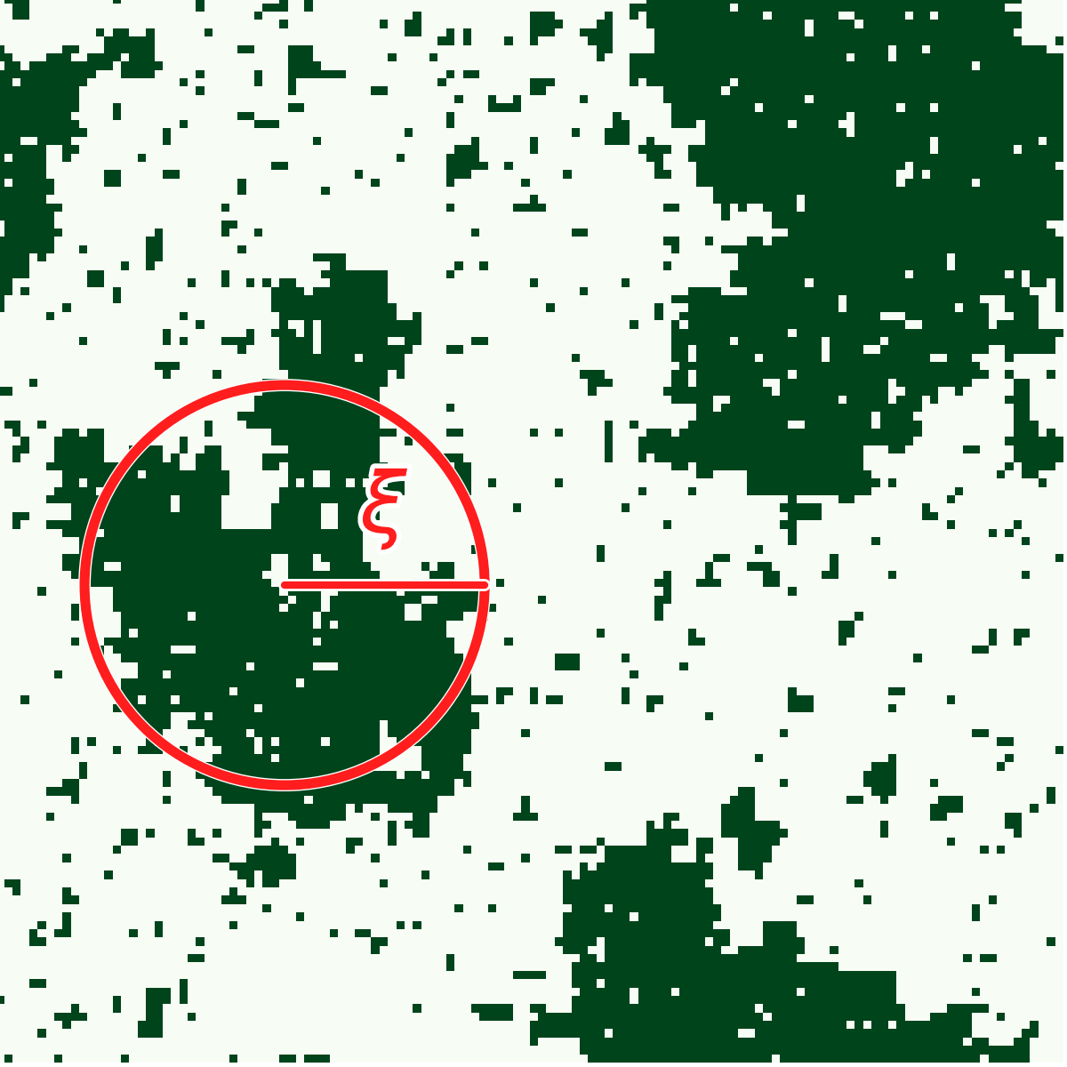
Although the magnetisation measures the degree of global order, there still could be order on smaller scales. This “local” order is captured by the correlation length ξ. Roughly, this measures the distance at which spins are correlated, in the sense that they have a high probability of being both up or down. For example in the image on the left, the correlation length is roughly the radius of the red circle: although the total magnetisation is zero, there is local order on scales of order ξ.

Data Sonification

Data sonification is the practice of transforming data into audio. Its objective is to communicate aspects of that data through the medium of sound.

In this project, the aim is to understand phase transitions, but also to perceive them from a visual/auditory perspective. Visualising the Ising Model is straightforward, as each microscopic state can be represented with a 2d grid of white and green pixels. Translating the state of the system into sound instead requires a mapping. In this mapping lies the art of data sonification.

The mapping is constructed such that the statistical properties of the model are reflected by its sound: each spin plays a fixed note whose pitch is higher/lower if the spin is “up”/“down”. The decay and detunement are controlled by the amount of disagreement with its neighbours, such that a spin that disagrees is short and detuned. The correlation length is then mapped to the cutoff frequency of a low pass filter, such that the degree of local order controls the overall brightness. In this way, the overall sound emerges from the interaction rules between many simple voices.

Let us now understand and listen to the different phases that occur in this model.

Conclusions

We started from a glass of water and the expectation that small causes produce small effects. The Ising Model shows how this expectation breaks down: a single, local rule, in which each spin prefers to agree with its neighbours, is enough to produce distinct phases of matter and abrupt transitions between them. None of these phases is written into the rule itself: they emerge from the interaction of many spins, and only become visible, or audible, at the scale of the whole lattice.

Listening to the model gives these ideas a different texture. Disorder is heard as a neurotic arpeggio, order as a harmonic pad whose octave reveals which way the symmetry has been broken, and a quench as a pad that never quite resolves. At the critical point, where the correlation length spans the entire grid, the sound is at its richest, because structure is present on every scale at once. This is also where physics is at its most surprising: near their critical points, systems as different as magnets and fluids share the same critical behaviour, a property known as universality. The Ising Model is a drastic simplification, but the phenomena it captures are real, and data sonification offers one more way to perceive them: with our ears as well as our eyes.